
* This blog post is an English translation of an article originally published in Japanese on April 4, 2025.
Introduction
As technologies like AR glasses, autonomous mobile robots, and drones that rely on cameras to perceive the real world continue to advance, the need for high-speed, high-accuracy Bundle Adjustment (BA) algorithms is increasing more than ever before.
The algorithms are essential for vSLAM (Visual Simultaneous Localization and Mapping) and SfM (Structure from Motion), both of which serve to estimate camera positions and reconstruct 3D point clouds in space.
The CoLi-BA (Compact Linearization-based Bundle Adjustment) algorithm, introduced by Z. Ye et al. in 2022, is one such algorithm that solves the BA problem.
CoLi-BA introduces several novel techniques to accelerate computation compared to conventional methods. It achieves this by compressing the Jacobian matrix to reduce computational complexity and optimizing memory access through strategic reordering of cameras and feature points, thereby minimizing cache miss rates. Indeed, it is reported to be 2 to 5 times faster than widely used methods such as g2o and Ceres without significant loss of accuracy.
In this article will first formulate the BA problem, then explain the computational steps of CoLi-BA, and finally outline the methods that contribute to its speedup.
Problem Formulation
The BA problem has also been introduced in the Tech blog “Speeding up Bundle Adjustment with CUDA and Source Code Release(Japanese only),” but here we will provide a formulation more aligned with the notation in the paper.
Suppose there is a point cloud \({\boldsymbol P} =
\{p_j \in {\mathbb R}^3 \mid 1 \leq j \leq n_p\}\) in three-dimensional space, and this is captured by a set of cameras \({\boldsymbol C}
= \{c_i \mid 1 \leq i \leq n_c\}\). Using the position \(t_i \in {\mathbb R}^3\) and rotation matrix \(R_i \in \mathcal{M}_{3\times
3}(\mathbb{R})\) of camera \(c_i\), the coordinates \(z_{ij} \in {\mathbb R}^2\) when \(p_j\) is captured are obtained as follows:
- \(q_{ij} = R_i(p_j – t_i)\) (Apply rotation \(R_i\) to the relative coordinates from \(t_i\))
- Draw a line passing through the origin and \(q_{ij}\), and let \(z_{ij}\) be the xy components of its intersection with the \(z=1\) plane. (That is, calculate \((x,y,z) \mapsto (x/z,y/z)\) for each point)
Conversely, given the captured coordinates \(z_{ij}\), we can consider the problem of finding the point cloud and camera poses that would generate them. The BA problem is to derive the original \(P, C\), given \(\tilde{z}_{ij} = z_{ij} + \epsilon_{ij}\), which includes measurement error \(\epsilon_{ij}\), as input. More specifically, the goal is to find \({\boldsymbol C}, {\boldsymbol P}\) that minimize the following cost function:
\[f({\boldsymbol C}, {\boldsymbol P}) = \sum_{1\leq i \leq n_c} \sum_{1
\leq j \leq n_p} \frac{1}{2} ||\epsilon_{ij}||^2\]
This problem is a non-linear least squares problem, and well-known algorithms exist. This article will not delve deeply into these methods themselves but will explain how CoLi-BA speeds up the necessary computations: “calculating the Hessian matrix of \(f\)” and “calculating the Schur complement (discussed later).” For more details on solving non-linear least squares problems, please refer to the Tech blog “Speeding up Bundle Adjustment with CUDA and Source Code Release.”
Approximation of the Jacobian Matrix
To calculate the Hessian matrix, we first need to obtain an expression for the Jacobian matrix.
The Jacobian matrix of \(\epsilon_{ij}\), corresponding to the three inputs (camera rotation, camera position, point position), is denoted as \(J_{ij} = \begin{pmatrix}J_{ij}^\phi &
J_{ij}^t & J_{ij}^p\end{pmatrix}\).
Note: Here, \(\phi_i\) is a 3-dimensional vector, and \(\frac{\partial}{\partial
\phi_i}\) corresponds to “partial differentiation with respect to rotation around the axis \(\phi_i\).” This correspondence between a 3D vector and 3D rotation is known to be derivable by utilizing the fact that for a small 3D vector \(\omega\), the infinitesimal rotation matrix around \(\omega\) can be approximated as \(I+[\omega]_\times\). (Refer to “Infinitesimal Rotation” and “Composition of Rotations” at https://qiita.com/scomup/items/fa9aed8870585e865117). For a more detailed explanation, please refer to materials on Lie groups and Lie algebras.
Each part can be expressed as a product of two partial derivatives via \(q_{ij}\):
\[J_{ij}^\phi = \frac{\partial \epsilon}{\partial \phi_i} = \frac{\partial
\epsilon}{\partial q_{ij}}\frac{\partial q_{ij}}{\partial \phi_i}\]
\[J_{ij}^t = \frac{\partial \epsilon}{\partial t_i} = \frac{\partial
\epsilon}{\partial q_{ij}}\frac{\partial q_{ij}}{\partial t_i}\]
\[J_{ij}^p = \frac{\partial \epsilon}{\partial p_j} = \frac{\partial
\epsilon}{\partial q_{ij}}\frac{\partial q_{ij}}{\partial p_j}\]
The partial derivatives on the right side of each equation can be written as:
\[\frac{\partial q_{ij}}{\partial \phi_i} = -R_i[a_{ij}]_\times\]
\[\frac{\partial q_{ij}}{\partial t_i} = -R_i\]
\[\frac{\partial q_{ij}}{\partial p_j} = R_i\]
(where \(a_{ij}\) = \(p_j – t_i\), and \([a]_\times\) is the skew-symmetric matrix that maps \(v\) to \(a \times v\).)
On the other hand, for the calculation of the left-side partial derivative \(\frac{\partial
\epsilon}{\partial q_{ij}}\), approximating the measurement error by the deviation on the unit sphere projection, instead of the projection onto the \(z=1\) plane used in the original formulation, is expected to improve the properties of the matrices in the formulas and contribute to speedup. Specifically, with \(\tilde{x}_{ij} = (z_x, z_y,
1)\) (where \((z_x, z_y) =
\tilde{z}_{ij}\)), we approximate:
\[\epsilon_{ij} \simeq e_{ij} =
\frac{q_{ij}}{||q_{ij}||} –
\frac{\tilde{x}{ij}}{||\tilde{x}{ij}||}\]

By incorporating this approximation, the Jacobian matrix takes the following form:
\[J_{ij}^\phi = -R_i[\bar{a}_{ij}]\times\]
\[J_{ij}^t = -s_{ij}R_i(I-\bar{a}_{ij}\bar{a}_{ij}^\top)\]
\[J_{ij}^p = s_{ij}R_i(I-\bar{a}_{ij}\bar{a}_{ij}^\top)\]
(where \(s_{ij} = \frac{1}{||a_{ij}||},
\bar{a}{ij} = s{ij}a_{ij}\))
The properties of the matrices appearing in these equations:
- Orthogonality of \(R_i\) (inverse is transpose)
- Expression of \([\bar{a}_{ij}]\times\) using cross product
- Expression of \(I – \bar{a}_{ij}\bar{a}_{ij}^\top\) using projection
- will contribute to speeding up the construction of the Hessian and Schur complement later.
Hessian Matrix
Next, let’s consider the Hessian matrix of the cost function \(f\). Let \(N_c = 6n_c, N_p =
3n_p\). The size of the Hessian matrix is \((N_c + N_p) \times (N_c + N_p)\).
The specific expression is derived from the Jacobian matrix. We define the following small Hessian blocks:
\[H_i^{cc} = \sum_j {J_{ij}^c}^\top J_{ij}^c\]
\[H_j^{pp} = \sum_i {J_{ij}^p}^\top J_{ij}^p\]
\[H_{ij}^{cp} = {J_{ij}^c}^\top J_{ij}^p\]
(where \(J_{ij}^c =
\begin{pmatrix}J_{ij}^\phi & J_{ij}^t\end{pmatrix} \in
\mathcal{M}_{3 \times 6} (\mathbb{R})\))
Furthermore, we construct block diagonal matrices \(A =
\text{diag}(H_1^{cc}, \cdots, H_{n_c}^{cc})\) and \(B = \text{diag}(H_1^{pp}, \cdots,
H_{n_p}^{pp})\), and a block matrix \(D =
(H_{ij}^{cp})\). Then, the overall Hessian matrix can be written as:
\[H = \begin{pmatrix} A & D \\ D^\top& B
\end{pmatrix}\]
Here, the rotation matrices that appeared in the Jacobian can be eliminated in the Hessian expression. Taking \(H_j^{pp}\) as an example, after some algebraic manipulations, we get: \(\sum_i
s_{ij}^2 (I – \bar{a}_{ij}\bar{a}_{ij}^\top)^\top (I –
\bar{a}_{ij}\bar{a}_{ij}^\top)\) and indeed, \(R_{ij}\) does not appear.
The expression can be further simplified. Noting that \((\bar{a}_{ij}\bar{a}_{ij}^\top)^2 =
\bar{a}_{ij}(\bar{a}_{ij}^\top\bar{a}_{ij})\bar{a}_{ij}^\top =
\bar{a}_{ij}\bar{a}_{ij}^\top\), we have: \((I – \bar{a}_{ij}\bar{a}_{ij}^\top)^\top (I –
\bar{a}_{ij}\bar{a}_{ij}^\top) = I – 2\bar{a}_{ij}\bar{a}_{ij}^\top +
(\bar{a}_{ij}\bar{a}_{ij}^\top)^2 = I –
\bar{a}_{ij}\bar{a}_{ij}^\top\)
Furthermore, from the cross product property \(\bar{a}_{ij} \times (\bar{a}_{ij} \times x) =
(\bar{a}_{ij}^\top x)\bar{a}_{ij} – (\bar{a}_{ij}^\top \bar{a}_{ij})x =
(\bar{a}_{ij}\bar{a}{ij}^\top -I)x\), it follows that \(I – \bar{a}_{ij}\bar{a}_{ij}^\top =
-[\bar{a}_{ij}]\times^2\).
Finally, it turns out that \(H_j^{pp}\) can be expressed in the very simple form: \(-s_{ij}^2[\bar{a}_{ij}]\times^2\).
By performing similar calculations for all Hessian blocks, and using the vector \(\hat{a}_{ij} = s_{ij}\bar{a}_{ij}\), the following expressions can be shown:
\[H_i^{cc} = \sum_j \begin{pmatrix}
-[\bar{a}_{ij}]\times^2 & -[\hat{a}_{ij}]\times \\
[\hat{a}_{ij}]\times & -[\hat{a}_{ij}]\times^2
\end{pmatrix}\]
\[H_j^{pp} = \sum_i -[\hat{a}_{ij}]\times^2\]
\[H_{ij}^{cp} = \begin{pmatrix}
[\hat{a}_{ij}]\times \\
[\hat{a}_{ij}]\times^2
\end{pmatrix}\]
Schur Complement
Finally, using the Hessian matrix, we calculate the Schur complement. In the algorithm, we need to find the solution \(H\varDelta x = b\), using the Hessian matrix \(H\) and some large vector b.
This is generally a computationally intensive process, but fortunately, we know a lot about the structure of H. In particular, if H can be expressed in the form \(H =
\begin{pmatrix} A & D \\ D^\top& B\end{pmatrix}\), then by using the Schur complement \(A – D B^{-1} D^\top\), \(\varDelta x\) can be calculated without explicitly computing the inverse of the entire \(H\). (For details, please refer to the “Structure of the Coefficient Matrix” section in this Tech blog(Japanese only).)
In this calculation, since \(B\) is a block diagonal matrix, the computation of \(D’ := D
B^{-1}\) is relatively fast. The bottleneck is the calculation of \(D’ D^\top\), the product of two large sparse matrices.
If we define each block of \(D’D^\top\) as \(d_{i_1 i_2} \in \mathcal{M}_{3\times
3}(\mathbb{R})\), it can be calculated as:
\[d_{i_1i_2} = \sum_j H_{i_1j}^{cp}(H_j^{pp})^{-1}(H_{i_2j}^{cp})^\top\]
Here, using the aforementioned skew-symmetric matrix representation of the Hessian blocks can significantly reduce the amount of computation. For example, multiplying a \(6\times 3\) matrix by a \(3\)-dimensional vector normally requires 18 multiplications. However, the result of multiplying the matrix \(H_{ij}^{cp}\) from the right by a vector \(x\) can be computed with 2 cross products (12 multiplications) using:
\[H_{ij}^{cp} x = \begin{pmatrix}\hat{a}_{ij} \times x \\ \hat{a}_{ij}
\times (\hat{a}_{ij} \times x)\end{pmatrix}\]
With such optimizations, it can be confirmed that the number of floating-point multiplications required for each \(j\) in the above equation drops from 162 to 108.
Ordering Strategy
The speedup techniques so far have focused on reducing the number of operations and memory usage through error approximation. On the other hand, CoLi-BA also implements speedups focused on hardware characteristics, specifically by determining a computation order that suppresses cache misses.
In real-world datasets, it is assumed that many camera-observation point pairs have no dependency (the observation point is not visible to the camera). The structure of matrix \(D\) can be represented as an \(N_c \times N_p\) matrix tiled with Hessian blocks between cameras and observation points. However, the Hessian sub-matrices for non-dependent pairs are zero matrices, so \(D\) is expected to be quite sparse. (This tendency is expected to be stronger as the number of cameras increases.)
Reiterating the formula for calculating each block \(d_{ij}\) of \(D’D^\top\):
\[d_{i_1i_2} = \sum_j H_{i_1j}^{cp}(H_j^{pp})^{-1}(H_{i_2j}^{cp})^\top\]
Here, by only considering \(j\) for which \(H_{i_1j}^{cp}\) is non-zero, the number of operations is reduced. This is a calculation method that leverages the sparsity of \(D\) and is already well-utilized in existing methods. In addition to this speedup, CoLi-BA proposes determining the order of \(i_1\) such that the values of \(H_j^{pp}\) and \(H_{i_2j}^{cp}\) referenced in the previous \(i_1\) iteration are likely to remain in cache.
Specifically, for each camera \(i\), let \(b^r_i :=\{j \mid H_{ij}^{cp} \neq
O\}\) (the set of points observed by camera i). The problem is formulated as finding a permutation \((o_1, …, o_{n_c})\) of \((1, …, n_c)\) that minimizes \(\sum |b^r_{o_i} \cap b^r_{o_{i+1}}|\). The rows of the matrix are reordered according to the obtained sequence \((o_i)\).
This problem can be equated to finding the minimum Hamiltonian path in an undirected graph with \(n_c\) vertices. Therefore, finding an exact solution is difficult, and CoLi-BA determines the order from an approximate solution using a simple greedy method.
Measurement Results
In the original paper, measurements were performed on 25 test cases of various sizes selected from KITTI and 1DSfM, with experimental results showing a 5x speedup compared to Ceres and a 2x speedup compared to g2o.
We also ran experiments using the program released by the paper’s authors on a 12-core CPU (2.2 GHz).
Additionally, we prepared 10 test cases created by dumping the BA inputs calculated when running ORB-SLAM2 with data such as KITTI as input.
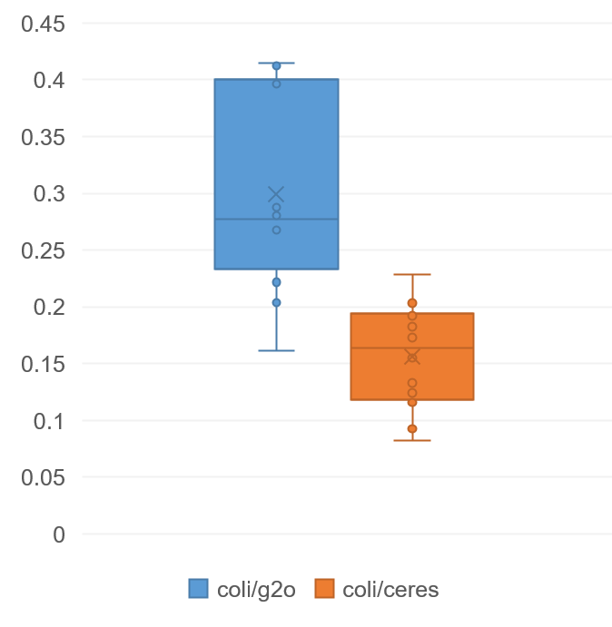
Figure 1 plots the ratio of CoLi-BA’s execution time to that of the other two methods for each test case. On average across all test cases, CoLi-BA takes about 0.3 times the time of g2o and about 0.15 times the time of Ceres.
Furthermore, since CoLi-BA uses approximations for errors, it is necessary to evaluate whether the resulting error significantly deviates from existing methods.
For each observation point, the smaller the magnitude of the difference \(\epsilon_{ij} = \hat{z}_{ij} – z_{ij}\) between the actual observed coordinates (\(z_{ij}\)) and the theoretical observed coordinates projected from the obtained 3D coordinates (\(\hat{z}_{ij}\)), the smaller the error. The paper used Mean Squared Error
\[\text{MSE} = \displaystyle \frac{1}{n_c n_p}\sum_{1\leq i \leq n_c}
\sum_{1 \leq j \leq n_p} ||\epsilon_{ij}||^2\]
for error evaluation, so we follow that here.
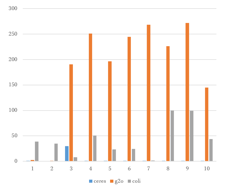
Figure 2 plots the Mean Squared Error for CoLi-BA, g2o, and Ceres for each test case, ordered from left to right by test case size (number of cameras). For some small cases, CoLi-BA’s error is observed to be larger than existing methods, but for medium-sized test cases, g2o’s error spikes, resulting in an order of Ceres < CoLi-BA < g2o. Since such large differences in error were not observed in the test case suite used in the paper, these results suggest that the performance of the methods may depend on the characteristics of the test cases (e.g., relatively few cameras).
References
- Z. Ye, G. Li, H. Liu, Z. Cui, H. Bao and G. Zhang, “CoLi-BA: Compact Linearization based Solver for Bundle Adjustment,” in IEEE Transactions on Visualization and Computer Graphics, vol. 28, no. 11, pp. 3727-3736, Nov. 2022, doi: 10.1109/TVCG.2022.3203119.
- g2o: https://github.com/RainerKuemmerle/g2o
- ceres: https://github.com/ceres-solver/ceres-solver