Evaluating LLM Fine-tuning Efficiency on NVIDIA RTX 6000 Blackwell Max-Q

This article is a guest post by Yuki Maeda, who worked with us as an intern.

He investigated the execution speed and memory consumption required for LLM fine-tuning using the latest GPU, the NVIDIA RTX PRO 6000 Blackwell Max-Q.

Article Summary

This article demonstrates the following:

1. Empirical Evaluation of Fine-tuning Methods, Speed, and Memory Efficiency

• Investigated efficient LLM fine-tuning techniques such as LoRA and QLoRA, alongside Unsloth, a library optimized for speed and VRAM efficiency.
• Conducted performance benchmarks on the NVIDIA RTX 6000 Blackwell Max-Q using Qwen3-8B, Qwen3-32B, and GPT-OSS-120B.
• Achieved up to a 3x speedup and ~80% memory reduction using Unsloth compared to standard LoRA.
• Successfully fine-tuned the 120B parameter model (GPT-OSS-120B) on a single GPU workstation.

2. Superiority of the NVIDIA RTX PRO 6000 Blackwell Max-Q GPU

• Compared the time required for fine-tuning between the NVIDIA RTX PRO 6000 Blackwell Max-Q and the H100 SXM5. Qwen3-32B and GPT-OSS-120B were used for the comparison (Qwen3-8B was omitted as its training time is particularly short and it shares the same architecture as Qwen3-32B).
• While the H100 SXM5 was faster for Qwen3-32B, the NVIDIA RTX PRO 6000 Blackwell Max-Q was faster for GPT-OSS-120B.
• It was revealed that the characteristics of the NVIDIA RTX PRO 6000 Blackwell Max-Q—namely its cost-performance, large memory, and low power consumption—make it particularly suitable for scenarios where fine-tuning is performed while keeping workstation operational costs low.

---

Introduction

Hello. I am Maeda, an intern.

Methods for making LLMs respond based on the latest information or specialized knowledge include fine-tuning and RAG. Among these, the strengths of fine-tuning include:

• Potential for reduced latency, as there is no need for external search intervention like in RAG.
• The ability to customize not only knowledge injection but also the model’s output format, tone, and behavior.

On the other hand, the weaknesses of fine-tuning include:

• It requires significant time for training and necessitates more memory than inference.
• Frequent fine-tuning is required for the LLM to maintain up-to-date knowledge, which incurs costs in terms of time and power. Especially in situations where fine-tuning is conducted daily, it is desirable for a single session to complete sufficiently fast (within a limited timeframe, such as overnight).

Therefore, considering situations where one wants to perform fine-tuning on an inference GPU or reflect the latest knowledge by fine-tuning a local LLM, performing fine-tuning with minimal time and memory is essential. In this article, I will first introduce general efficiency methods for LLM fine-tuning and provide specific code examples.

Furthermore, at Fixstars, we have adopted the NVIDIA RTX PRO 6000 Blackwell Max-Q (hereafter abbreviated as 6000 Blackwell Max-Q) for our AIStation. This is a relatively new GPU, and facts such as:

• “How many parameters can a model have to be fine-tuned on a single 6000 Blackwell Max-Q?”
• “What scale of dataset can be used to complete fine-tuning of an existing model within a specified time?”

are not yet well-established. Therefore, we will experimentally confirm the answers to these questions by actually performing LLM fine-tuning on the 6000 Blackwell Max-Q under varying conditions. Finally, through a comparison with NVIDIA’s other architecture, the H100, we will consider how the hardware features of the 6000 Blackwell Max-Q (cost-performance, memory size, low power) are leveraged for LLM applications.

---

Prerequisite Knowledge 1: Fine-tuning Acceleration Technologies

What is PEFT?

Generally, updating all parameters of a model during fine-tuning (full fine-tuning) requires an enormous amount of time and memory. Especially with the rapid increase in model parameters in recent years, full fine-tuning is not a realistic strategy.

The approach used instead is PEFT (Parameter-Efficient Fine-Tuning). PEFT is a general term for fine-tuning methods that reduce the amount of computation by training only a portion of the total parameters while maintaining performance comparable to full fine-tuning. While I will omit details here, various methods exist within PEFT, many of which are supported by the Hugging Face PEFT library [1].

What is LoRA?

LoRA (Low-Rank Adaptation) [2] is a type of PEFT and is widely used for its memory efficiency and ability to maintain high performance.

Instead of updating all parameters, LoRA adds a small adapter 𝐵𝐴—a product of “low-rank matrices”—to the weight matrix 𝑊, and only this adapter is trained (the weights of 𝑊 are frozen during training). If the weight after fine-tuning is 𝑊, then 𝑊 is represented by the formula 𝑊’ = 𝑊 + 𝐵𝐴. Specifically, the difference in the weight matrix updated by fine-tuning is represented not by a matrix of the same size as the original weight  𝑊∈ℝ^𝑑×𝑘, but by the product of low-rank matrices  𝐴∈ℝ^𝑟×𝑘 and 𝐵∈ℝ^𝑑×𝑟 (where  𝑟≪
min⁡(𝑘,𝑑), and only the weights of 𝐴 and 𝐵 are trained.

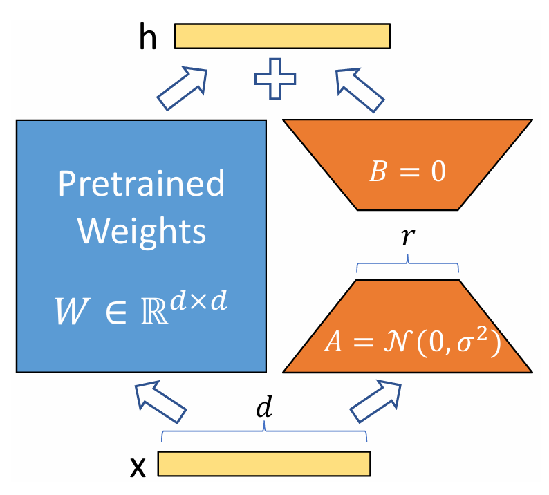
One major benefit of LoRA is the significant reduction in the number of parameters to be trained. If the weight matrix 𝑊 were updated directly, the number of parameters would be 𝑑𝑘; however, when training only 𝐴 and 𝐵, it can be reduced to (𝑑+𝑘)𝑟 ≪𝑑𝑘. Since reducing the number of parameters also reduces the time required for training, LoRA is an efficient method in terms of both training time and memory consumption.

Furthermore, since the parameters of the entire original model are frozen and only the weights of the additional small matrices 𝐴 and 𝐵 are trained, switching models for each task is easy. That is, when executing multiple different tasks (e.g., summarization, Q&A, translation) with the same base model 𝑊, one only needs to save the pairs of small 𝐴 and 𝐵 (adapter files) trained for each task and switch them dynamically during inference. If one were to naively update the original model’s parameters without using LoRA, the entire model would need to be saved for each task, consuming a massive amount of memory.

What is QLoRA?

QLoRA (Quantized LoRA) [3] is, simply put, a fine-tuning method that achieves further reduction in memory usage by combining LoRA with quantization. In QLoRA, the weights of the original model are kept in GPU memory quantized to a low precision of 4-bit. This reduces memory consumption by the model weights to about 1/4 compared to loading weights at 16-bit precision (FP16 or BF16).

Note that these 4-bit model weights are dequantized as needed during inference and gradient calculation (they are not calculated in 4-bit). Due to this dequantization process, some reports suggest that fine-tuning with QLoRA takes slightly longer than with LoRA.

Additionally, QLoRA achieves efficient memory management through technologies such as Double Quantization and Paged Optimizers. A more detailed explanation of the QLoRA implementation is provided in the Appendix.

About Unsloth

Unsloth [4] is a Python library designed for accelerating and reducing the memory footprint of LLM fine-tuning. The name is a portmanteau implying “un-sloth” (not slow like a sloth).

According to the official documentation [4], it implements unique custom kernels using the Triton language (a language developed by OpenAI that allows writing complex GPU kernels with simple Python-like syntax). By performing efficient gradient and LoRA calculations through its own implementation, it achieves a 2x improvement in training speed and a 70% reduction in memory consumption compared to implementations not using Unsloth. It also supports LoRA and QLoRA, enabling even faster and more memory-efficient fine-tuning. A more detailed explanation of Unsloth’s optimization is provided in the Appendix.

Note:

As of November 2025, an error appeared when trying to use the Unsloth library on the 6000 Blackwell Max-Q in the author’s environment. In this case, building Xformers from source as indicated solved the problem. Also, the official Unsloth documentation has a page explaining environment setup for Blackwell, so please refer to that as well.

---

Prerequisite Knowledge 2: What kind of GPU is the 6000 Blackwell Max-Q?

As mentioned earlier, Fixstars has adopted the 6000 Blackwell Max-Q for AIStation. While a detailed performance investigation was introduced in another article, here we highlight points highly relevant to LLM fine-tuning. Additionally, while the previous article compared it with the H100 PCIe, this experiment used the H100 SXM5 (a higher-performance version), so we compare performance with the H100 SXM5 again here.

First, the 6000 Blackwell Max-Q can be described in one word as a GPU with excellent cost-performance. Since H100 SXM5 is a server GPU and its price is rarely public, citing the comparison from the previous article: the H100 PCIe is approximately 4.7 million JPY [5], whereas the 6000 Blackwell Max-Q is 1.6 million JPY [6].

Summarizing part of the theoretical computing performance and memory bandwidth:

Metric	6000 Blackwell Max-Q	H100 SXM5
Architecture	Blackwell (GB202)	Hopper (GH100)
FP64 (TFLOPS)	1.7	33.5
FP32 (TFLOPS)	109.7	66.9
TF32 (TFLOPS)	438.9	989.4
BF16 (TFLOPS)	877.9	1978.9
FP4 (TFLOPS)	3511.4	N/A
Memory Bandwidth (GB/sec)	1792	3352

From this table, it is clear that the H100 SXM5 has higher performance, except for FP32, INT32, and FP4, which is hardware-supported for the first time in the Blackwell architecture. On the other hand, in terms of performance per unit price, the 6000 Blackwell Max-Q often wins.

A particularly noteworthy feature of the 6000 Blackwell Max-Q regarding LLM fine-tuning is its large memory capacity. While the H100 SXM5 has 80GB, the 6000 Blackwell Max-Q is equipped with 96GB of memory. This makes it possible to perform not only inference but also fine-tuning on a single GPU using the efficient methods mentioned above.

In terms of power consumption, the 6000 Blackwell Max-Q is also superior. While the H100 SXM5 is 700W, the 6000 Blackwell Max-Q is 300W, which is kept low—a characteristic well-suited for workstations.

---

Measurement Method

As stated, we will evaluate fine-tuning performance on the 6000 Blackwell Max-Q. First, let’s cover the measurement method.

Machine Specs:

• GPU: 6000 Blackwell Max-Q (VRAM: 97,887 MiB)
• CPU: Intel(R) Xeon(R) w5-2455X (12 cores)
• Memory: 251 GiB
• OS: Ubuntu 22.04 / CUDA: 13.0 / Python: 3.10.12

Models Used:

1. Qwen3-8B
2. Qwen3-32B
3. GPT-OSS-120B

Datasets Used:

1. dataset 1: japanese_alpaca_data (https://huggingface.co/datasets/fujiki/japanese_alpaca_data): This is a Japanese translation of the Alpaca dataset (https://huggingface.co/datasets/tatsu-lab/alpaca)and is an instruction-following dataset. Average input token count: 117 (after truncation with max_seq_length=2048).
2. dataset 2: wikipedia_ja (https://huggingface.co/datasets/wikimedia/wikipedia): This is a dataset of Japanese Wikipedia articles. Since we required a dataset with a longer average input token count, we set the article body as the input and the article title as the output, training the model to predict the title from the body text. However, as Wikipedia articles often follow a format where the first sentence begins with “[Title] is…”, we programmatically removed the first sentence before training to eliminate unnecessary simplicity and ensure a more challenging task. Average input token count: 861 (after truncation with max_seq_length=2048).

For both datasets, we performed a shuffle and extracted a subset of 1,000 samples (due to time constraints) for fine-tuning and subsequent measurements.

---

Fine-tuning Code Used for Measurements

Below is the actual code used for fine-tuning GPT-OSS-120B with Unsloth. Comments have been added to explain hyperparameters that significantly impact fine-tuning speed. For details on other settings, please refer to the Unsloth LoRA Hyperparameters Guide.

Module Imports

Python

import torch
from unsloth import FastLanguageModel
from transformers import TrainingArguments
from datasets import load_dataset
from trl import SFTTrainer
from transformers.trainer_callback import TrainerCallback
import pandas as pd
import time
import os

Logger Definition

To monitor training progress and memory consumption, the following logger was defined:

Python

class GpuMemoryLoggerCallback(TrainerCallback):
    def __init__(self, log_file="gpu_memory_log.csv"):
        self.log_file = log_file
        self.log_data = []
        self.start_time = None

    def on_train_begin(self, args, state, control, **kwargs):
        self.start_time = time.time()
        os.makedirs(os.path.dirname(self.log_file), exist_ok=True)
        if not os.path.exists(self.log_file):
            df_header = pd.DataFrame(columns=[
                "step", "epoch", "elapsed_time_sec",
                "progress_ratio", "memory_allocated_gb",
                "memory_reserved_gb", "peak_memory_gb"
            ])
            df_header.to_csv(self.log_file, index=False)

    def on_step_end(self, args, state, control, **kwargs):
        if not torch.cuda.is_available():
            return
        log_interval = 10
        if state.global_step % log_interval == 0 or state.global_step == state.max_steps:
            elapsed_time = time.time() - self.start_time
            memory_allocated = torch.cuda.memory_allocated(0) / (1024**3)
            memory_reserved = torch.cuda.memory_reserved(0) / (1024**3)
            peak_memory = torch.cuda.max_memory_allocated(0) / (1024**3)
            log_entry = {
                "step": state.global_step,
                "epoch": state.epoch,
                "elapsed_time_sec": elapsed_time,
                "progress_ratio": state.global_step / state.max_steps,
                "memory_allocated_gb": memory_allocated,
                "memory_reserved_gb": memory_reserved,
                "peak_memory_gb": peak_memory,
            }
            self.log_data.append(log_entry)
            df = pd.DataFrame(self.log_data)
            df.to_csv(self.log_file, mode='a', header=False, index=False)
            self.log_data = []

Model Loading and LoRA Configuration

• unsloth/gpt-oss-120b-unsloth-bnb-4bit: An Unsloth-optimized model with 4-bit quantization to reduce footprint.
• max_seq_length = 2048: Limits the input to 2048 tokens, affecting both speed and memory.
• r = 8: The rank for LoRA adapters; impacts memory and final model performance.
• use_gradient_checkpointing = "unsloth": Enables Unsloth’s custom implementation to save VRAM during backpropagation.

Python

model_id = "unsloth/gpt-oss-120b-unsloth-bnb-4bit"
output_dir = "./results_gpt-oss-120b_unsloth"
max_seq_length = 2048

model, tokenizer = FastLanguageModel.from_pretrained(
    model_name = model_id,
    max_seq_length = max_seq_length,
    dtype = None,
    load_in_4bit = True,
)

model = FastLanguageModel.get_peft_model(
    model,
    r = 8,
    target_modules = ["q_proj", "k_proj", "v_proj", "o_proj", "gate_proj", "up_proj", "down_proj"],
    lora_alpha = 16,
    lora_dropout = 0,
    bias = "none",
    use_gradient_checkpointing = "unsloth",
    random_state = 3407,
)

Dataset Configuration

The function formatting_function_alpaca converts the loaded Alpaca-format data (instruction, input, output) into a single chat-format text that the LLM can understand. The internal implementation of this function should be adjusted according to the specific dataset being used.

Python

def formatting_function_alpaca(example, tokenizer):
    instruction = example["instruction"]
    input_text = example.get("input", "")
    output_text = example["output"]
    if input_text:
        user_content = f"{instruction}\n{input_text}"
    else:
        user_content = instruction
    messages = [
        {"role": "user", "content": user_content},
        {"role": "assistant", "content": output_text}
    ]
    text = tokenizer.apply_chat_template(
        messages,
        tokenize=False,
        add_generation_prompt=False
    )
    return {"text": text}

dataset = load_dataset("fujiki/japanese_alpaca_data", split="train")
dataset = dataset.shuffle(seed=42)
subset_size = 1000
dataset = dataset.select(range(subset_size))
dataset = dataset.map(
    formatting_function_alpaca,
    remove_columns=dataset.column_names)

Trainer Configuration

The following code sets up the training environment.

• num_train_epochs: Specifies the number of training epochs.
• per_device_train_batch_size: Specifies the batch size. Increasing this value improves training speed but increases GPU memory consumption.
• gradient_accumulation_steps: Used to increase the effective batch size. While it saves memory, it can slow down training.

Python

training_args = TrainingArguments(
    output_dir=output_dir,
    num_train_epochs=1,
    per_device_train_batch_size=16,
    gradient_accumulation_steps=1,
    optim="adamw_torch",
    logging_steps=10,
    learning_rate=2e-4,
    fp16=False,
    bf16=True,
    max_grad_norm=0.3,
    save_strategy="epoch",
)

trainer = SFTTrainer(
    model=model,
    tokenizer=tokenizer,
    train_dataset=dataset,
    args=training_args,
    callbacks=[GpuMemoryLoggerCallback(log_file=unsloth_log_file)]
)

Executing Training

Python

trainer.train()
trainer.model.save_pretrained("./result/gpt-oss-120b_unsloth_adapter")

Inference Method After Fine-tuning

Here is how to perform inference using the fine-tuned LoRA adapter.

Python

import torch
from unsloth import FastLanguageModel
from peft import PeftModel

# Define the response generation function
def generate_response(model_to_use, instruction, input_text=""):
    if input_text:
        user_content = f"{instruction}\n{input_text}"
    else:
        user_content = instruction
    
    messages = [{"role": "user", "content": user_content}]
    prompt = tokenizer.apply_chat_template(
        messages,
        tokenize=False,
        add_generation_prompt=True
    )
    
    inputs = tokenizer(prompt, return_tensors="pt").to(DEVICE)
    outputs = model_to_use.generate(
        **inputs,
        max_new_tokens=1024,
        do_sample=True,
        temperature=0.7,
        top_k=50,
        top_p=0.95
    )
    
    return tokenizer.decode(outputs[0], skip_special_tokens=True)

# Test cases for evaluating capabilities
test_cases = [
    {
        "instruction": "Explain why the sky is blue to a primary school student.",
        "input": "",
        "name": "Knowledge & Simple Explanation"
    },
    {
        "instruction": "Change the following sentence to the passive voice.",
        "input": "She writes a new poem every day.",
        "name": "Grammar Processing"
    },
    {
        "instruction": "I cool hot things and warm cold things. I breathe constantly, but have no lungs. What am I?",
        "input": "",
        "name": "Logical Reasoning"
    }
]

# Loading and Evaluation
BASE_MODEL_ID = "unsloth/gpt-oss-120b-unsloth-bnb-4bit"
ADAPTER_PATH = "./result/gpt-oss-120b_unsloth_adapter_alpaca"
DEVICE = "cuda" if torch.cuda.is_available() else "cpu"
OUTPUT_FILE = "unsloth_output.txt"

with open(OUTPUT_FILE, "w", encoding="utf-8") as f:
    # evaluate base model
    base_model, tokenizer = FastLanguageModel.from_pretrained(
        model_name = BASE_MODEL_ID,
        max_seq_length = 2048,
        dtype = torch.bfloat16,
        load_in_4bit = True,
    )
    base_model = FastLanguageModel.for_inference(base_model)
    base_model.eval()
    print("start base model evaluation...")

    f.write("\n" + "="*60 + "\n")
    f.write("  RESULTS: Base Model (GPT-OSS-120B) \n")
    f.write("="*60 + "\n\n")
    for case in test_cases:
        response_base = generate_response(base_model, case["instruction"], case["input"])
        f.write(f"--- Test Case: {case['name']} ---\n")
        f.write(f"Instruction: {case['instruction']}\n")
        if case['input']:
            f.write(f"Input: {case['input']}\n")
        f.write(f"Base Response:\n{response_base}\n\n")

    # evaluate LoRA fine-tuned model
    lora_model = PeftModel.from_pretrained(base_model, ADAPTER_PATH)
    lora_model = FastLanguageModel.for_inference(lora_model)
    lora_model.eval()
    print("start LoRA evaluation...")

    f.write("="*60 + "\n")
    f.write("  RESULTS: Fine-Tuned Model (LoRA) \n")
    f.write("="*60 + "\n\n")
    for case in test_cases:
        response_lora = generate_response(lora_model, case["instruction"], case["input"])
        f.write(f"--- Test Case: {case['name']} ---\n")
        f.write(f"Instruction: {case['instruction']}\n")
        if case['input']:
            f.write(f"Input: {case['input']}\n")
        f.write(f"LoRA Response:\n{response_lora}\n\n")

---

Measurement Results

All experiments in this section were conducted on a single machine equipped with one RTX 6000 Blackwell Max-Q.

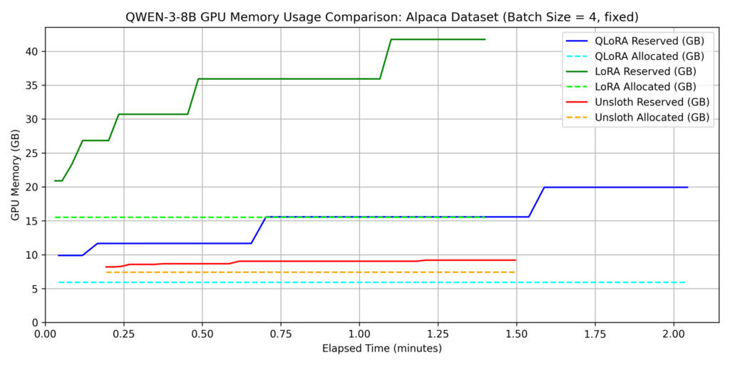
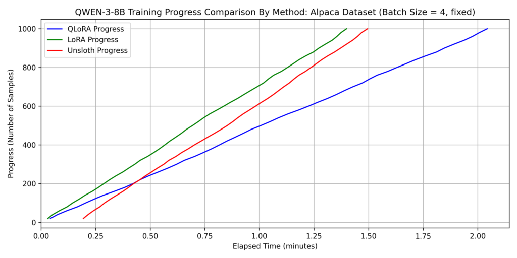
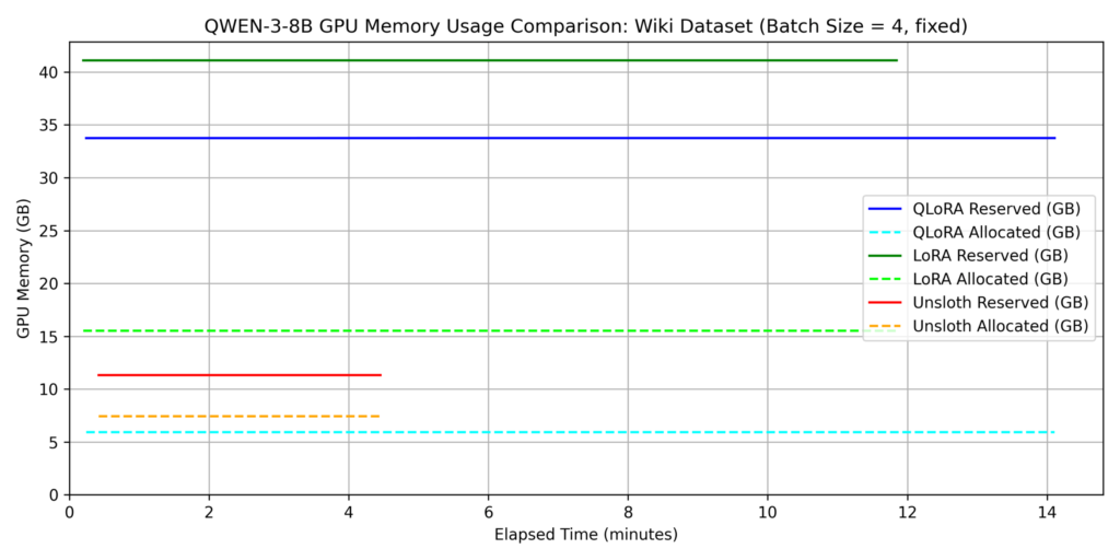
1. Comparison of Fine-tuning Methods for Qwen3-8B

We evaluated three methods: LoRA, QLoRA, and QLoRA with Unsloth (hereafter “Unsloth”). For this section, batch_size=4 was used for all methods.

dataset 1: japanese_alpaca_data

dataset 2: wikipedia_ja

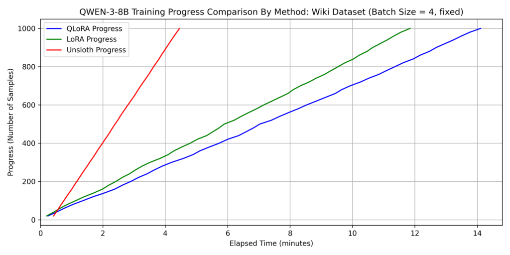
Key Findings on Training Time:

• QLoRA without Unsloth was the slowest across both datasets.
• For Dataset 2, Unsloth was over 3x faster than other methods.
• While QLoRA training time increased 7x from Dataset 1 to Dataset 2, Unsloth only saw a 3x increase. This suggests Unsloth’s efficient attention implementation works better as sequence length increases. Since self-attention complexity is  O(𝐿²) relative to sequence length 𝐿, it becomes the dominant factor for longer inputs.

Note: Unsloth requires more time during the first training cycle. This is likely due to the JIT (Just-In-Time) compilation overhead of custom Triton kernels during the first function call.

Key Findings on Memory Consumption:

• Compared to standard LoRA, QLoRA reduced allocated memory by approximately 1/3 (refer to the QLoRA section for why it isn’t 1/4).
• Unsloth significantly reduced the gap between allocated and reserved memory, indicating superior memory management. Specifically, in Dataset 1, reserved memory for Unsloth was roughly 80% lower than standard LoRA.

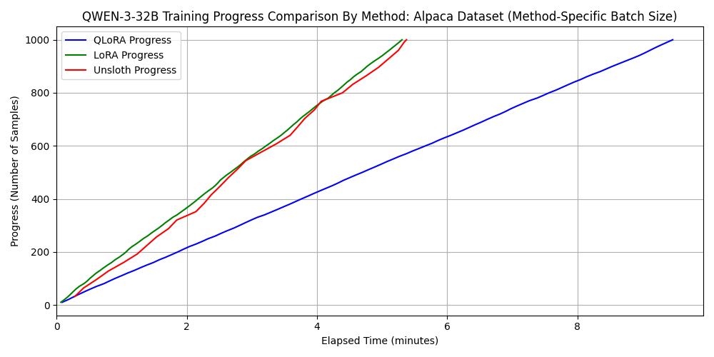
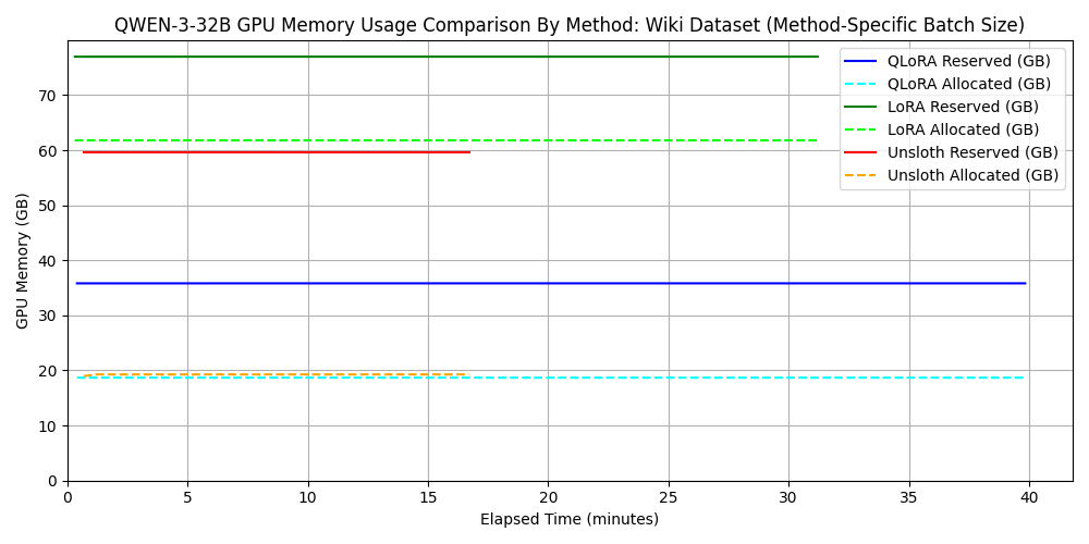
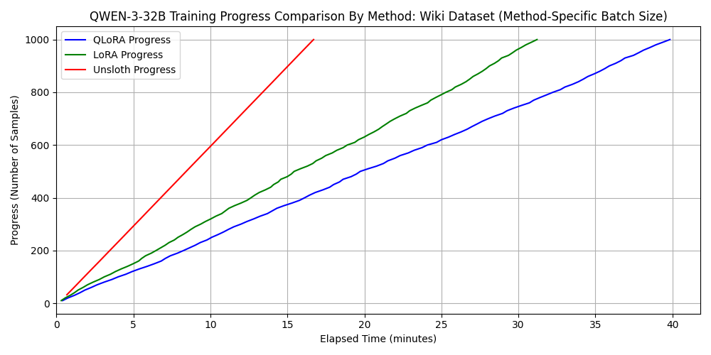
2. Comparison for Qwen3-32B

For standard LoRA/QLoRA, batch_size=4 exceeded the 96GB VRAM, so we used batch_size=2. However, Unsloth worked fine even with batch_size=32. This demonstrates that memory-efficient frameworks allow for larger batch sizes, improving parallelism and shortening training time.

dataset 1: japanese_alpaca_data

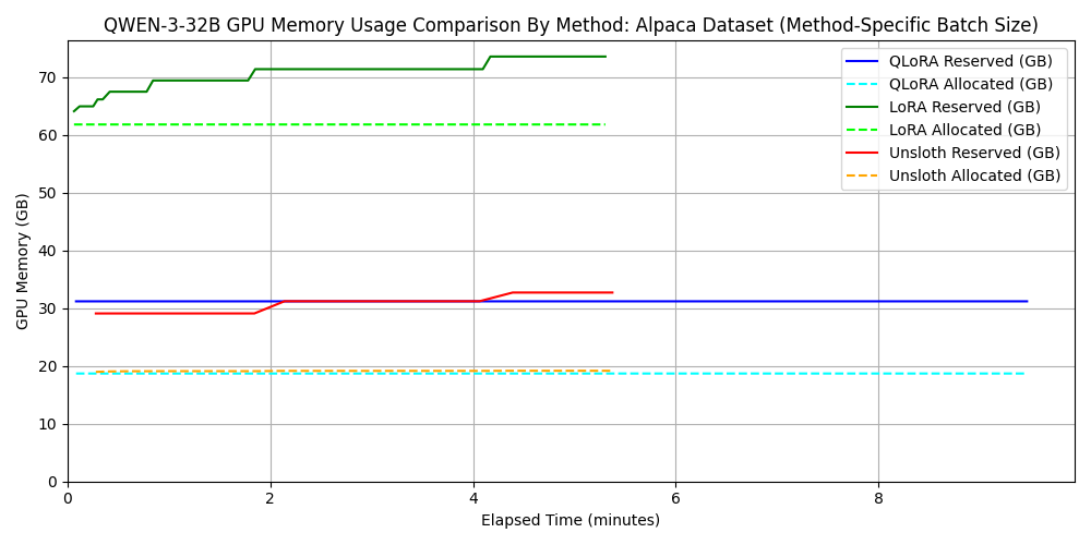
dataset 2: wikipedia_ja

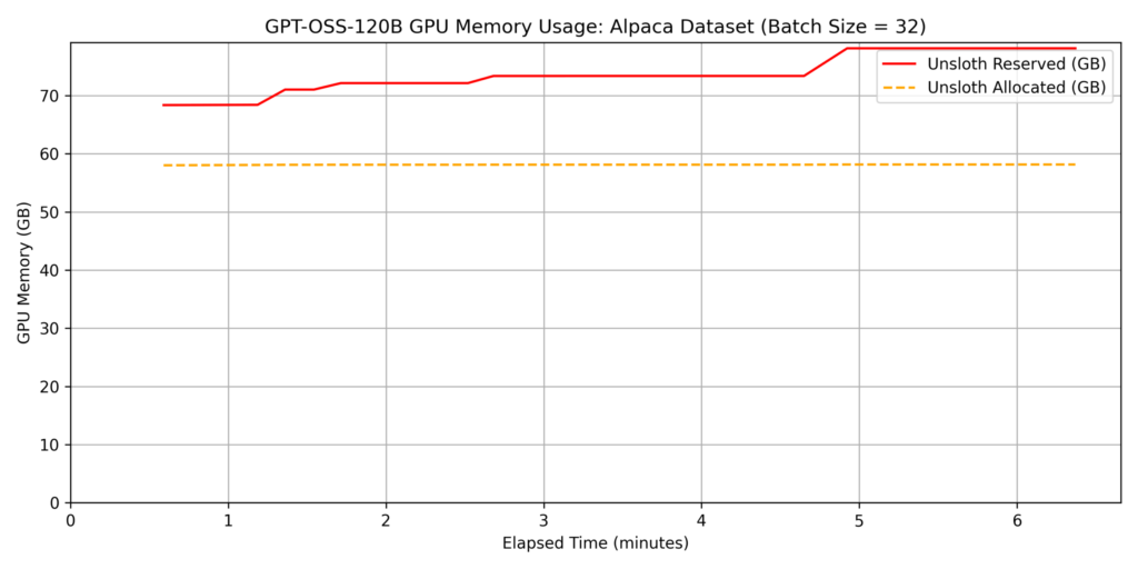
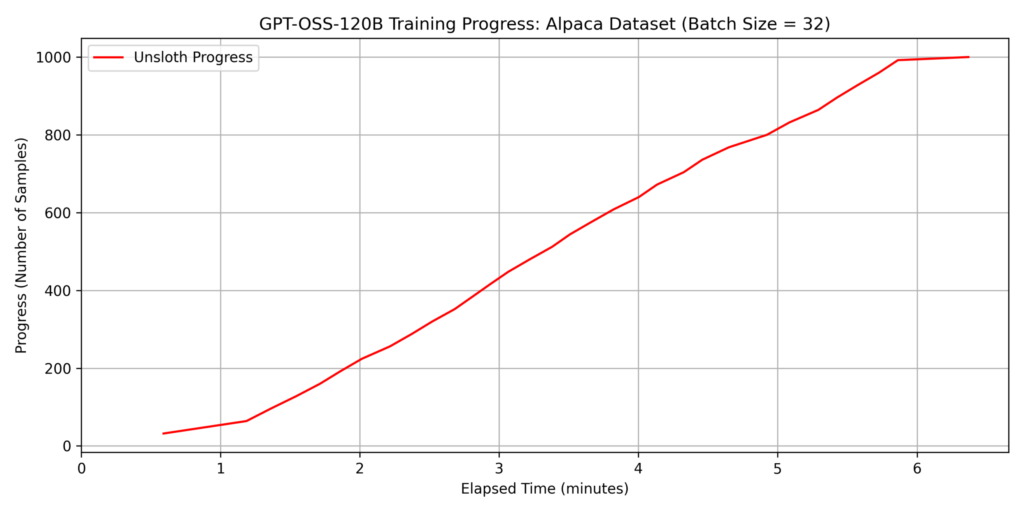
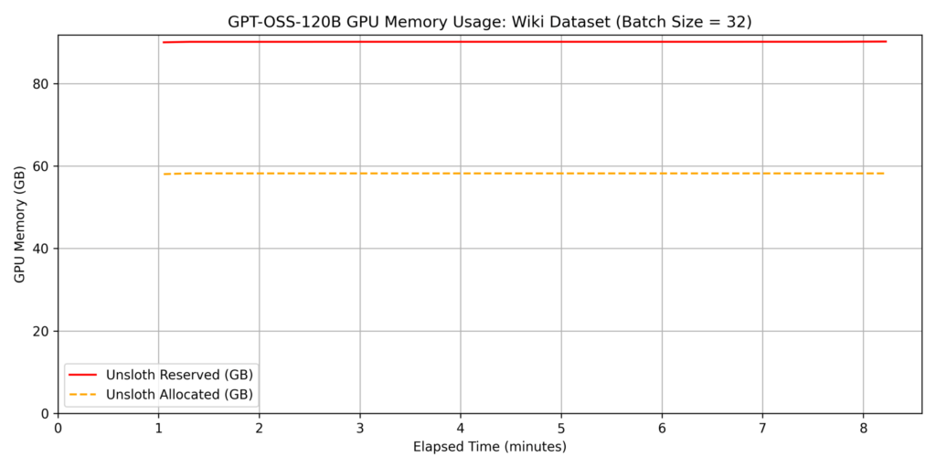
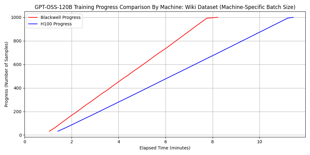
3. Performance evaluation of fine-tuning for GPT-OSS-120B

The previous experiments demonstrated Unsloth’s efficiency in memory management and speed. Building on these results, we evaluated the performance of fine-tuning GPT-OSS-120B, a model with a much larger parameter count.

Fine-tuning such a massive model is typically impossible on a single GPU with 96GB of VRAM using standard implementations; however, Unsloth’s memory optimization allowed us to fit the process within the 6000 Blackwell Max-Q’s capacity. For this test, we set the batch size to batch_size=32.

dataset 1: japanese_alpaca_data

dataset 2: wikipedia_ja

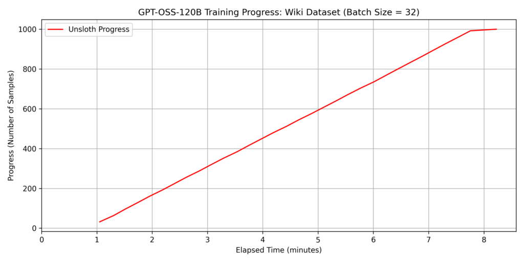
Note: The sudden drop in the slope at the end of the graph is because we trained a 1,000-sample dataset with a batch_size=32, resulting in only 8 samples remaining for the final cycle.

Note: When comparing the fine-tuning times of GPT-OSS-120B and Qwen3-32B, the training time for Qwen3-32B was actually longer, despite having fewer parameters. Upon checking the “Trainable parameters” displayed by Unsloth during training, we found the following:

• Qwen3-32B: 67,108,864 of 32,829,232,128 (0.20% trained)
• GPT-OSS-120B: 5,971,968 of 116,835,128,640 (0.01% trained)

As shown, GPT-OSS-120B has fewer trainable parameters. This aligns with a reported issue “[Bug] GPT OSS: No adapters for the experts?”. It appears that for MoE (Mixture-of-Experts) models like GPT-OSS-120B, even if “gate_proj”, “up_proj”, and “down_proj” are included in the target modules, only the attention layers are currently being trained.

While fine-tuning such a large model on a single GPU is usually difficult, Unsloth’s efficient memory management ensures it fits within the 96GB VRAM of the 6000 Blackwell Max-Q. For datasets with token lengths similar to Dataset 2, we found it possible to train approximately 5,000 samples per hour.

Qualitative Observation: Changes in Model Response

We also verified the change in model responses before and after fine-tuning. For this, we used the wikipedia_ja dataset (2,500 samples), as it makes changes in response format easier to observe. As mentioned earlier, the model was trained to predict the “article title” (output) based on the “Wikipedia article body minus the first sentence” (input). We expected the post-fine-tuning model to output specific nouns described in the article.

Example Input and Responses

Input:

“A group of people who distinguish themselves from others with a sense of fellowship. The scope of society is very broad, ranging from partial societies such as single organizations and associations to the entire society encompassing citizens… If there is a collection of certain humans where continuous communication and interaction take place, and these are ordered to some degree (this phenomenon is called social control) and organized, it can be considered a society…”

Pre-Fine-tuning Response:

“The text you provided is an explanation of the concept of ‘Society’, its scope, and its components. Below is a summary for better understanding:

1. Basic Definition of Society: A group of people who share a sense of fellowship…
2. Scope of Society (Scale): (omitted)…”

Post-Fine-tuning Response:

Example Input and Responses

Input:

“A group of people who distinguish themselves from others with a sense of fellowship. The scope of society is very broad, ranging from partial societies such as single organizations and associations to the entire society encompassing citizens… If there is a collection of certain humans where continuous communication and interaction take place, and these are ordered to some degree (this phenomenon is called social control) and organized, it can be considered a society…”

Pre-Fine-tuning Response:

“The text you provided is an explanation of the concept of ‘Society’, its scope, and its components. Below is a summary for better understanding:

1. Basic Definition of Society: A group of people who share a sense of fellowship…
2. Scope of Society (Scale): (omitted)…”

Post-Fine-tuning Response:

Society

This confirms that the model’s response format successfully shifted to match the dataset format—specifically, providing short nouns like Wikipedia titles.

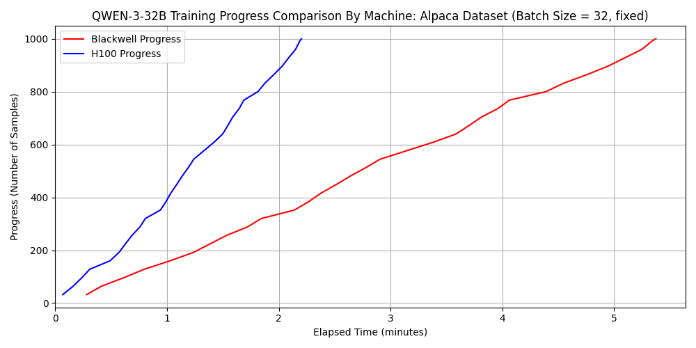
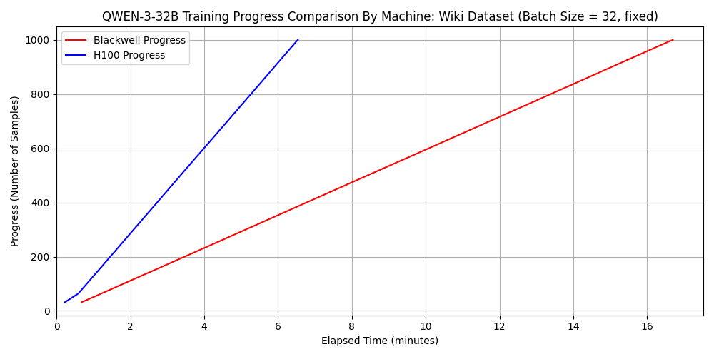
4. Comparison between 6000 Blackwell Max-Q and H100 SXM5

Next, we shift our perspective to compare the fine-tuning speeds of the 6000 Blackwell Max-Q and the H100 SXM5. The specifications of the machine equipped with the H100 SXM5 used for comparison are as follows:

• GPU: NVIDIA H100 80GB HBM3 (VRAM: 81,559 MiB)
• CPU: Intel(R) Xeon(R) Platinum 8480+ (56 cores / 2 sockets)
• Memory: 2.0 TiB
• PCIe Generation: 5
• OS: Ubuntu 22.04 / CUDA: 12.8 / Python: 3.10.12 / Docker: 28.4.0

Comparison Conditions:

• Evaluations were conducted using Unsloth, as it is the most speed- and memory-efficient implementation.
• Two models were used: Qwen3-32B and GPT-OSS-120B (Qwen3-8B was excluded due to its extremely short training time and architectural similarity to Qwen3-32B).
• Datasets used were Dataset 1 and Dataset 2, as described previously.
• The batch size was generally set to batch_size=32. However, for the combination of H100, GPT-OSS-120B, and Dataset 2, batch_size=16 was used because the VRAM was insufficient.

Comparison Results for Qwen3-32B

Comparison Results for GPT-OSS-120B

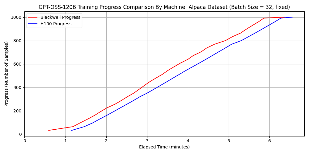
Surprisingly, for the combination of GPT-OSS-120B and Dataset 2, the 6000 Blackwell Max-Q was approximately 1.3 times faster than the H100 SXM5. Considering that the H100 SXM5 has superior FP16 and BF16 arithmetic performance, this result might seem counterintuitive.

Analysis of the Results

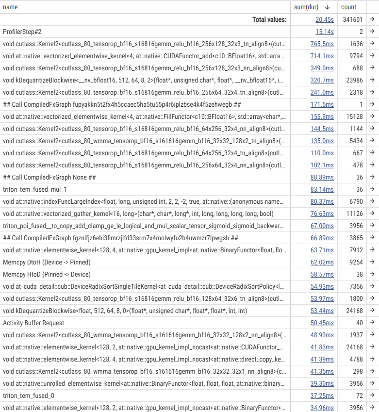
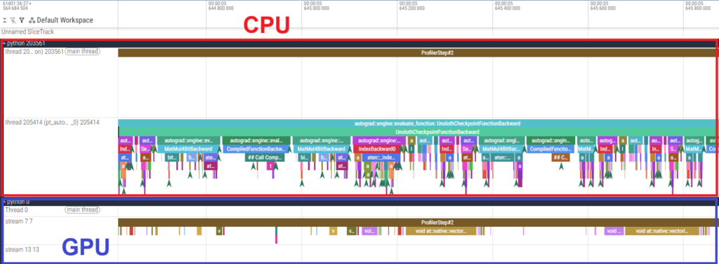
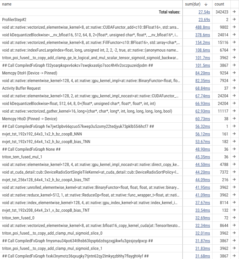
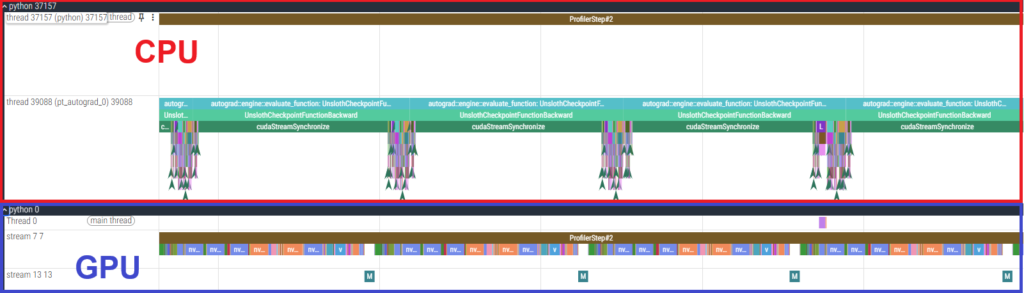
To investigate the cause, we used the PyTorch Profiler to analyze the fine-tuning of GPT-OSS-120B. Below are the execution time tables for each kernel and a timeline snippet of the backward pass.

• Results of 6000 Blackwell Max-Q

• Results of H100 SXM5

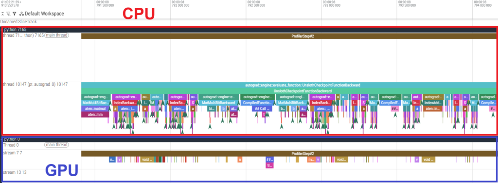
The execution time tables show that the actual GPU processing time for individual kernels is shorter on the H100 SXM5. However, the timeline reveals large gaps between GPU kernels, indicating that the GPU is “idling” while waiting for the CPU. In other words, the process is CPU-bound.

To further verify this, we used Nsight Systems to check the kernel activity time (indicated in light blue).

• Results of 6000 Blackwell Max-Q

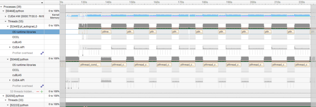
• Results of H100 SXM5

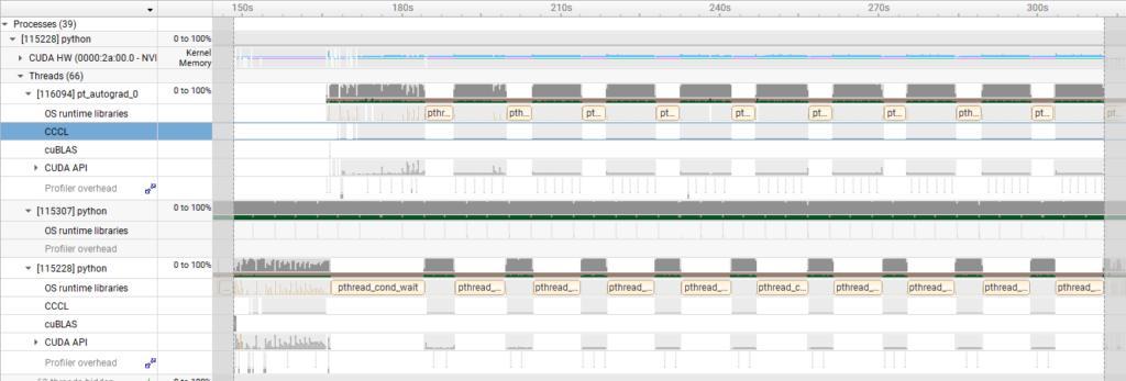
These visualizations confirm that the H100 SXM5 experienced significantly longer GPU idle time, meaning the CPU processing became a bottleneck. This is considered the primary cause of the difference in execution time observed for the GPT-OSS-120B.

Furthermore, we conducted profiling for the Qwen3-32B using the PyTorch Profiler, which revealed that the GPU was utilized almost constantly, as shown in the figure below. Unlike the MoE model, the Qwen3-32B is a dense model with a larger number of trainable parameters. Consequently, the increased GPU processing load made the task GPU-bound. This explains why the H100 SXM5, with its superior raw arithmetic performance, achieved higher speeds in this specific case.

• Results of 6000 Blackwell Max-Q

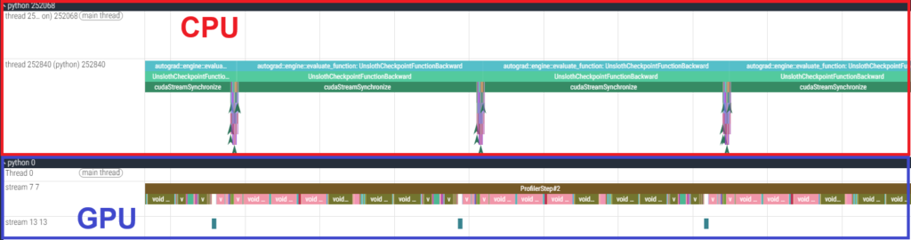
• Results of H100 SXM5

Discussion: Advantages of 6000 Blackwell Max-Q in LLM Fine-tuning

What specific advantages does the 6000 Blackwell Max-Q offer for LLM fine-tuning?

First and foremost, its primary appeal is affordability. While it is natural that the 6000 Blackwell Max-Q (targeted at workstations) and the H100 SXM5 (targeted at data centers) differ in price due to their different intended uses, there is roughly a three-fold difference in cost. If the 6000 Blackwell Max-Q is sufficient for your requirements, it is the logical choice.

Next, let’s consider the fine-tuning time. When fine-tuning relatively sparse models like GPT-OSS-120B, the 6000 Blackwell Max-Q can actually be faster, as demonstrated above. In such cases, the 6000 Blackwell Max-Q holds an advantage in both speed and cost. On the other hand, the H100 SXM5 leads in raw speed for models like Qwen3-32B. To put this into perspective, we calculated the number of dataset samples that can be fine-tuned per hour:

Number of dataset samples fine-tunable per hour for qwen3-32b

	dataset 1	dataset 2
6000 Blackwell Max-Q	11000	3600
H100 SXM5	27000	9200

Number of dataset samples fine-tunable per hour for gpt-oss-120b

	dataset 1	dataset 2
6000 Blackwell Max-Q	9400	7300
H100 SXM5	9200	5200

A typical workstation use case might involve “updating internal AI data overnight, outside of working hours.” If you have an 8-hour window, you can process eight times the amounts shown above. Whether the 6000 Blackwell Max-Q is “sufficient” depends on your specific dataset size. If a single machine can handle your scale, its cost-effectiveness makes it a highly compelling option.

Furthermore, the large memory size of the 6000 Blackwell Max-Q has a direct impact on LLM fine-tuning. Memory capacity dictates which models can be loaded; for instance, GPT-OSS-120B requires approximately 30 GB for weights alone, even with 4-bit quantization. Consequently, the 6000 Blackwell Max-Q allows for fine-tuning a wider variety of models on a single GPU compared to existing workstation GPUs. Beyond just “fitting” the model in VRAM, the larger memory also enables larger batch sizes. This increases training parallelism and improves effective processing speed. As shown in our tests, the 6000 Blackwell Max-Q can sometimes utilize batch sizes that the H100 SXM5 cannot, contributing to overall acceleration.

Finally, regarding power consumption: as mentioned previously, the maximum power draw is 700 W for the H100 SXM5, whereas the workstation-oriented 6000 Blackwell Max-Q is kept low at 300 W. In the case of GPT-OSS-120B fine-tuning, the 6000 Blackwell Max-Q is superior not only because it uses less power but also because it completes the task faster. This is a significant advantage for workstation deployment.

In summary, the 6000 Blackwell Max-Q is particularly well-suited for scenarios where fine-tuning must be performed while minimizing operational costs in a workstation environment.

Conclusion

To recap, this article has demonstrated the following:

1. Experimental measurements of fine-tuning methods, speed, and memory consumption

• Researched fine-tuning LLMs using efficient methods such as LoRA and QLoRA, and investigated the use of the Unsloth library for high-speed, memory-efficient training.
• Experimentally evaluated the execution speed and memory efficiency of the 6000 Blackwell Max-Q using Qwen3-8B, Qwen3-32B, and GPT-OSS-120B.
• With Unsloth, we achieved up to 3x speedup and approximately 80% memory savings compared to standard LoRA.
• The acceleration effect of Unsloth was particularly significant for long text sequences.
• Using QLoRA and Unsloth, we successfully fine-tuned GPT-OSS-120B on a machine with a single 6000 Blackwell Max-Q.

2. Advantages of the 6000 Blackwell Max-Q GPU

• Compared fine-tuning times between the 6000 Blackwell Max-Q and the H100 SXM5.
• While the H100 SXM5 was faster for Qwen3-32B, the 6000 Blackwell Max-Q was faster for GPT-OSS-120B.
• The 6000 Blackwell Max-Q’s hallmark features—cost-performance, large memory, and low power consumption—make it an ideal choice for fine-tuning while keeping operational costs low in workstation environments.

---

References:

• [1] https://github.com/huggingface/peft
• [2] Edward J. Hu and Yelong Shen and Phillip Wallis and Zeyuan Allen-Zhu and Yuanzhi Li and Shean Wang and Lu Wang and Weizhu Chen, “LoRA: Low-Rank Adaptation of Large Language Models”
• [3] Tim Dettmers and Artidoro Pagnoni and Ari Holtzman and Luke Zettlemoyer, “QLoRA: Efficient Finetuning of Quantized LLMs”
• [4] https://docs.unsloth.ai/
• [5] AKIBA PC Hotline!編集部 オリオスペックが「NVIDIA H100 Tensor Core GPU」の受注開始、約471万円 (Japanese)
• [6] AKIBA PC Hotline!編集部 VRAM 96GB搭載の「NVIDIA RTX PRO 6000 Blackwell Max-Q Workstation Edition」が登場、約160万円 (Japanese)
• [7] https://www.nvidia.com/content/dam/en-zz/Solutions/design-visualization/quadro-product-literature/NVIDIA-RTX-Blackwell-PRO-GPU-Architecture-v1.0.pdf
• [8] https://resources.nvidia.com/en-us-hopper-architecture/nvidia-h100-tensor-c
• [9] https://huggingface.co/blog/RakshitAralimatti/learn-ai-with-me
• [10] https://github.com/unslothai/unsloth
• [11] https://github.com/unslothai/unsloth-zoo