
* This blog post is an English translation of an article originally published in Japanese on April 21, 2025.
Introduction
This is Hoshii, a part-time intern.
This article is a report on the results of the “Speeding up 3D Gaussian Splatting” task I worked on as an internship project.
In this article, I will introduce a method that sped up the rendering of the currently very hot 3D Gaussian Splatting technique by approximately 15%, along with its results. By optimizing the rendering with a focus on the “Mahalanobis distance,” we succeeded in improving processing speed without degrading image quality.
What is 3D Gaussian Splatting?
3D Gaussian Splatting for Real-Time Radiance Field Rendering is a method proposed in 2023. It enables high-speed, high-definition training and rendering (drawing) for Novel-view Synthesis.
While Neural Radiance Fields (NeRF), announced in 2020, had garnered attention for novel-view synthesis, 3D Gaussian Splatting demonstrates superior performance to NeRF in terms of training and rendering speed.
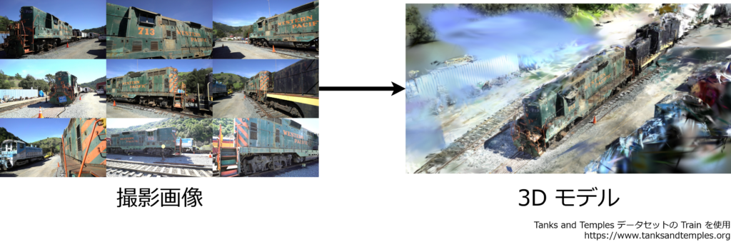
What is Novel-view Synthesis?
It estimates a 3D shape from multiple existing images to create a 3D model. Using the estimated 3D model, it renders images taken from new camera angles.
Features of 3D Gaussian Splatting
In 3D Gaussian Splatting, a 3D model is represented as a combination of 3D Gaussians.
The shape of a 3D Gaussian is defined by a 3D covariance matrix \(\Sigma\) and a center point \(\mathbf\mu\), expressed as: \(G(\mathbf x) = e^{-\frac{1}{2}(\mathbf x – \mathbf
\mu)^\top\Sigma^{-1}(\mathbf x – \mathbf \mu)}\)
Intuitively, each 3D Gaussian has a blurry ellipsoidal shape, as shown in the figure below.
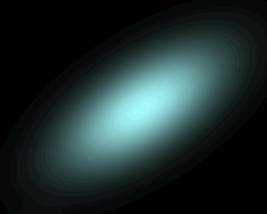
In addition to distribution information, 3D Gaussians also hold opacity and color information. Real-world objects can change their hue when viewed from different directions due to effects like light reflection. Color information is represented using spherical harmonics to express these view-dependent color changes.
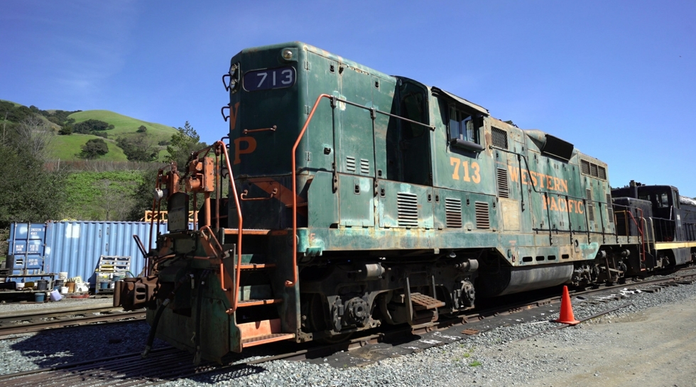
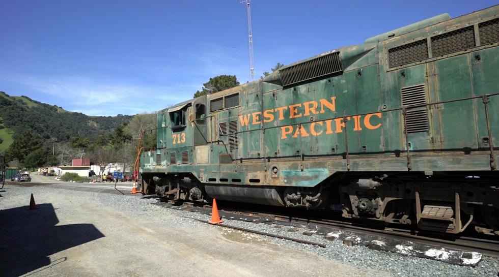
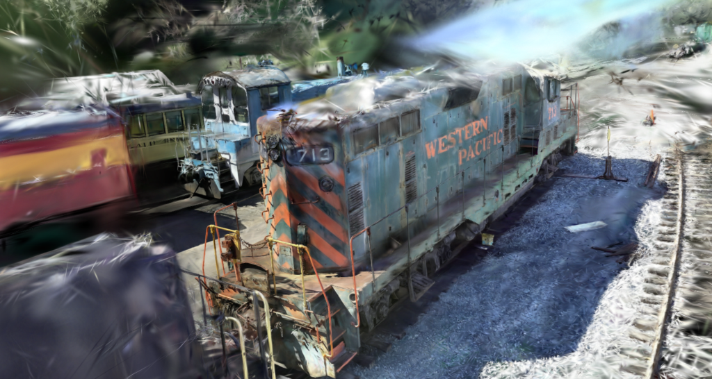
Models created with 3D Gaussian Splatting look good from a distance, but when viewed up close, it becomes apparent that they are an aggregate of 3D Gaussians, as shown in the figure below.

Rendering
In computer graphics, common methods for rendering images from 3D models include ray tracing and rasterization.
Ray tracing, as the name suggests, is a method that traces light rays. Light travels from a source to the camera or eye, reflecting off or refracting through multiple objects. This method calculates the color for each pixel on the image by tracing these light paths in reverse. Ray tracing can produce high-precision renderings but requires significant computation time, making it unsuitable for real-time processing.
3D Gaussian Splatting uses a rasterization approach. In rasterization, ray tracing is not performed; instead, objects in the 3D model are projected onto the image to determine the color of the pixels on the image. Because it can be processed quickly, rasterization is primarily used in applications requiring real-time processing, such as 3D games. In 3D Gaussian Splatting, rendering is performed by projecting each 3D Gaussian onto the image. Although it doesn’t involve calculations for light rays, 3D Gaussian Splatting can, as mentioned above, handle reflections to some extent by representing view-dependent color changes.
The output is a 3D model. Using this 3D model, images can be rendered from arbitrary viewpoints.
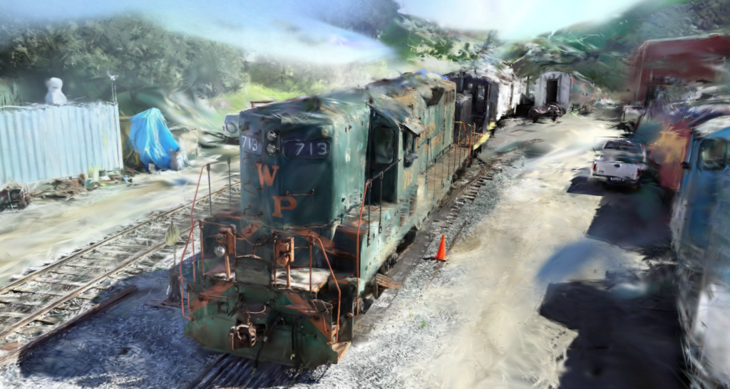
This dataset primarily features a green train, and the 3D shape of the green train is reconstructed with high precision. However, surrounding trains that are not frequently present in the images, or the ceiling parts of trains not included in the images, are not reproduced very well.
Speeding up 3D Gaussian Splatting
We performed speedup optimizations for 3D Gaussian Splatting. Specifically, we focused on optimizing the processing during rendering.
Speedup Method
Each 3D Gaussian is rendered as a blurry ellipse when projected onto the image. A characteristic of 3D Gaussians is that they are denser near the center and become sparser (or fainter) as you move away from the center. If a pixel is sufficiently far from the center, the influence of that 3D Gaussian becomes small enough to be negligible. Therefore, it’s effective to terminate the calculations for pixels that are beyond a certain distance.
In the original paper’s implementation, this calculation cutoff is already performed. However, the calculation range is quite wide. It sets the calculation range up to 3σ away from the center, based on the standard deviation σ in the major axis direction of the ellipse. Specifically, as shown in the figure below, the calculation range is the area contained within a square with sides of length 6σ, centered at the same point.
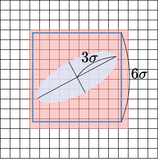
The influence on regions beyond \(3\sigma\) is at most about \(e^{-\frac{1}{2}\cdot 3^2}\approx 0.01\), so they likely considered it negligible. However, if we take this stance, it’s possible to narrow the calculation range further.
There is a concept called “Mahalanobis distance.” Mahalanobis distance is defined as \(d=\sqrt{(\mathbf x – \mathbf
\mu)^\top\Sigma^{-1}(\mathbf x – \mathbf \mu)}\) (where \(\mathbf{x}\), \(\mathbf{\mu}\), and \(\Sigma\) here are considered on the pixel coordinates projected onto the image). For pixels with the same Mahalanobis distance, the 3D Gaussian has the same influence. The Mahalanobis distance at a location \(3\sigma\) away in the major axis direction is \(3\). By calculating only for the range where the Mahalanobis distance is \(3\) or less, as shown in the figure below, the calculation range can be further reduced.

Verification
Verification Conditions
About the Implementation
We implemented and verified the method on OpenSplat, an open-source implementation of 3D Gaussian Splatting. OpenSplat has both CPU and GPU (CUDA) implementations; this time, we implemented the method for the GPU case. This part is implemented similarly in the original paper’s implementation.
Dataset
We used the Playroom dataset from Deep Blending for Free-Viewpoint Image-Based-Rendering. Out of 225 images, 205 were used for training and 20 for evaluation.
Execution Environment
CPU: Intel Core i7-14700, GPU: NVIDIA GeForce RTX 4060.
Results
We measured the time for 10,000 steps of execution.
The proposed method primarily speeds up the rendering part. Limiting the measurement to only the rendering part, the execution times were as follows:
| Method | Execution time per step (milliseconds) |
| Original implementation | 5.88 |
| Proposed method | 4.91 |
Compared to the original implementation, we succeeded in achieving approximately 15% speedup. Integrating this proposed method into a viewer can make it operate approximately 15% faster.
The overall execution times were as follows:
| Method | Execution time per step (milliseconds) |
| Original implementation | 33.4 |
| Proposed method | 32.1 |
Since the rendering part is not the bottleneck, the overall speedup was limited to about 4%.
Regarding image quality, we verified that there was no degradation using SSIM Loss on the 20 evaluation images.
| Method | SSIM Loss |
| Original implementation | 0.0312 ± 0.0095 |
| Proposed method | 0.0318 ± 0.0093 |
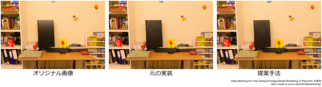
As shown in the table above, it was confirmed that no image quality degradation was observed. An example of the created images is shown below. It can be seen that there is no change in image quality between the original implementation and the proposed method.
Conclusion
I have introduced 3D Gaussian Splatting and described the speedup work I conducted as an internship project. 3D Gaussian Splatting is a relatively new paper published in 2023, but as of April 2025, it has already been cited over 3400 times and is a very hot research area.
Fixstars offers internships year-round. To all technical college, university, and graduate students, why not experience new technologies at Fixstars? Please see here(only in Japanese) for internship details.
Postscript
It turns out this speedup idea has been previously published: Speedy-Splat: Fast 3D Gaussian Splatting with Sparse Pixels and Sparse Primitives.